By Mark Elo
To begin with let us look at regular digital computers, or what physicists call a ‘Classical Computer’. This performs data processing tasks by manipulating bits; each bit can have a value of one or zero. A “Quantum” implementation of a computer manipulates quantum bits (Qubits). Qubits can have a value of one, zero or both simultaneously. When the bit is simultaneously a one and a zero, (yes one and zero at the same time, not oscillating quickly between two states) the bit is said to be in a state of superposition. Superposition is one of two key phenomena in Quantum Computing, the other being Entablement as they allow us to quickly crack encryption, make AI faster, model weather and the stock market.
In this article we will focus on Superposition. To understand this, we need to examine the properties of an electron, especially how electrons behave in the presence of electromagnetic (EM) fields and how this is used within Qubit. Consider Figure 1. Each atomic orbital is represented by an energy level measured in electron volts (eV), with the lowest orbit called the ground state. As a particle can also be a wave (Wave-particle duality), its energy level has a frequency equal to the energy level in eV divided by Planck’s constant (the quantization constant). If we want the electron to move to a higher energy state, we apply EM energy at a frequency equal to the desired energy level minus the current energy level, divided by Planck’s constant. The frequency and time the stimulus is applied is key, plus if we can constrain the energy levels to two, we have the fundamental building blocks for manipulating 1’s and 0’s with a single electron.
Electrons also possess a type of angular momentum called spin. As the electron moves from one energy level to another, the spin momentum changes. At the lower energy level, the momentum is pointing down, called the “spin-down.” When EM energy is applied, the spin changes until the momentum is pointing upwards as the electron achieves the next energy level. This is the “spin-up” state. When the electron state can be defined like this, it is said to possess an eigenstate, as both the position and momentum are known and can be quantified through measurement. We can say Spin-Up represents a logical 1, and Spin-down represents a Logical 0. So, we now have a Quantum implementation of a bit.
Now let’s make it a Qubit. As already discussed there exist possibilities that an electron can be in neither a spin-up or spin-down state, but in-between or a superposition of the two states. While superposition is fundamental to the operation of a quantum computer, we have what is referred to as the “measurement problem.” A state of superposition only can exist if you don’t “observe” it - the idea behind the popularized Schrödinger’s cat example. In a quantum system, observation is synonymous with measurement. As a physicist would say, the measurement causes the particle to be projected to one of its eigenstates or as an electronics engineer would say back to the logical 1 or 0.
There are many implementations of quantum bits, ranging from solid-state superconducting qubits to photon-based systems using lasers and modified crystals. In this article we will look at the Transmon solid-state implementation. A Transmon or Transmission Line Shunted Plasma Oscillation Qubit, is a type of solid-state qubit. Fundamentally, it is a tuned LC circuit connected to a transmission line, which resonates when an appropriate frequency is applied.
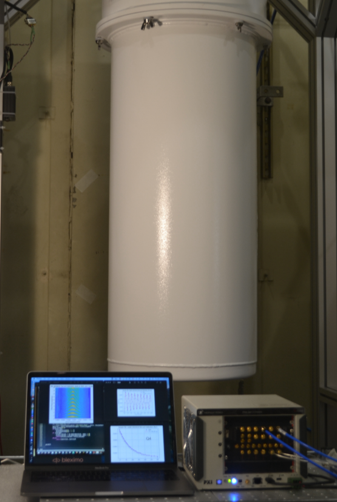
Figure 2 represents an actual Quantum System. As the spin and energy level change with the application of certain frequencies, a qubit is fundamentally based on several microwave resonant circuits connected via transmission lines, for both qubit control and measurement. The inductive component in an actual qubit is replaced with a Josephson junction. While still fundamentally an LC structure, this modifies the inductive properties of the circuit so only two resonant or energy states can occur - since the system must be constrained to two levels 1 and 0. The circuit is packaged in a protective shield with the RF connectors exposed, then is cooled to about -450°F to ensure the system exhibits Quantum behavior.
One of the key behaviors to establish for a Quantum Bit is to determine its resonant characteristics and determine at what frequencies it will exhibit Quantum behavior. The Q of the resonator is usually very high so the experimentalists will want to sweep a range of frequencies through the devices operating range to determine the exact resonant frequency.
Once the resonance is known we need to determine if the device exhibits quantum behavior. This is established with the Rabi Oscillation Measurement. If a frequency for a specific amount of time is applied, a pulse, you can make the electron move from the ground state to the exited state, and back again. This is often also referred to as a rotation, with the exited state being 180 degrees of rotation and back to the ground state 360 degrees of rotation. A physicist often refers to the pulse of durations Pi, 2Pi or even Pi/2. Pi as the time it takes to rotate the electron 180 degrees and 2Pi 360 degrees. In the Rabi oscillation measurement, we vary the pulse width to determine the exact length of Pi.
So now we know the exact resonant frequency and the time it takes the electron to Spin-up and Spin-down. The next step is to determine how long the device can maintain quantum behavior. This is the Relaxation Time measurement. To do this we apply a pulse of time length Pi, and steadily move the readout further and further away from the pulse to produce a decay curve. This is a true quality metric for Qubits, as the longer it can maintain a Quantum State the more effective it is at performing calculations. Figure 3 shows the Tabor Quantum Computing Measurement Control and Measurement System.
Quantum Computers, like all computers, utilize gates. While a Classical Computer utilizes NAND gates, built from transistors, Quantum Computer gates are realized from the electrical pulses with specific frequencies and lengths. A simplified example would be a ‘Not’ gate implementation, this would be the application of a Pi pulse or inverting the spin. We can add another gate to the sequence, the ‘Hadamard’ Gate or a Pi/2 pulse. As the Qubit is in a state of superposition at this point it is neither a 1 or 0, if we measure (or observe) the state of the Qubit, it will either snap to a 1 state or a 0 state. In an ideal world the probability of it snapping to each state would be equal, in real life interference from the outside world would cause the probability to be weighted one way or another.
With just two gates implemented on 5 Qubits, we can effectively create a 5-bit random number generator. Not much of an application, however we have not discussed the phenomenon of Entanglement yet. This allows us to connect multiple Qubits together utilizing the C-Not gate. Allowing for more complex algorithms and applications to be solved as discussed at the beginning of this article.
As we have discussed wave-particle duality, the photoelectric effect, electro magnetic resonance and probability are key elements in quantum computing. The manipulation of these phenomena creates various electron or photon spins that can ultimately help crack codes and facilitate secure communications, although there is still a long way to go! Today most quantum computing machines reside in research labs, with scientists trying to solve problems such as how longer a state of superposition can last (Relaxation) and reducing interference so more qubits can work together.
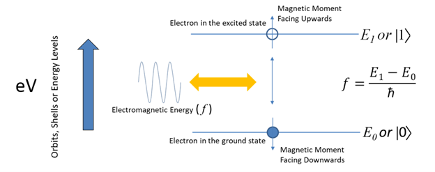
Figure 1: Electron Energy States
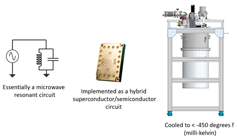
Figure 2: A Quantum Computer